

Key Takeaways
Use SQL to turn a question into a story the data can defend.
Start with curiosity. Anthony DeBarros learned SQL while covering USA Today’s weekly bestseller list. Searching sales, authors, and genres helped him spot patterns, from seasonal cookbook sales to the boost Oprah Winfrey gave featured writers. The point is not to collect clever commands. It is to ask a question, query evidence, and discover what the records can support.
Stories begin in tables. SQL, or Structured Query Language, retrieves, changes, and organizes data in databases. Unlike a spreadsheet limited to just over a million rows per sheet, a database can handle larger collections and related tables. The work still begins with a human question. SQL gives that curiosity a precise, repeatable way to investigate.
What's distinctive is the book's newsroom instinct: a query is not merely a technical operation, but a reporting question made testable. That orientation connects data analysis to investigative journalism, where a promising pattern is a lead, not yet a conclusion. The bestseller examples make this vivid because sales rankings can reveal cultural shifts while also tempting analysts to overinterpret a single week. A useful discipline is to separate the observation from its explanation: first establish what changed, then seek evidence for why. SQL can make a claim auditable, but it cannot make a weak question important.
Choose tables, keys, and data types that keep each value honest.
Give data a sound home. A relational database stores different kinds of things in separate tables and connects them with keys. In the school example, enrollment belongs in one table, student details in another, and a student ID links them. This avoids repeating a student’s name and birth date every time they enroll in a class, reducing both clutter and the risk of inconsistent edits.
Types carry meaning. Store dates as dates, money as exact decimals, and identifiers as text when their formatting matters. Census FIPS codes, for example, can begin with zero, which an integer would discard. Floating-point numbers can also introduce small calculation errors, making them a poor default for exact financial arithmetic.
Schema design is a form of preventive reasoning. A well-chosen type or key rules out entire classes of later mistakes, much as a measurement instrument constrains what can be recorded. The tradeoff is that a schema can also encode mistaken assumptions: a fixed name length, for example, may fail on an unusual but valid case. Good design therefore combines explicit rules with knowledge of how data is produced. The book’s distinction between a number and a code is especially useful: a value that looks numeric may function only as a label.
Interview a dataset before letting it answer your question.
Probe before concluding. DeBarros calls initial exploration “interviewing the data”: using queries to learn what the records contain, how complete they are, and whether values behave as expected. Start with selected columns, sorting, filters, distinct values, and counts. Then inspect ranges and missing entries. These simple checks can expose misspellings, odd dates, duplicate records, and fields that do not mean what their names suggest.
Documentation matters. In the library survey, negative visit counts were codes for nonresponse or a closed agency, not real negative visits. Summing them without checking the survey documentation would distort the total. A row count can also confirm an import: the 2019 county table should contain 3,142 records.
This practice resembles exploratory data analysis, where the first task is to understand distributions and possible measurement failures before fitting a model. It also has a governance dimension: missing values and unusual codes are decisions made by people or systems, not mere database quirks. In statistics, missingness can depend on the value being missing, which means deleting incomplete records may bias results. The book's advice to ask what a code means is stronger than simply flagging anomalies. A surprising value may be an error, a convention, or the most interesting fact in the dataset.
Join records on valid keys, then summarize at the right level.
Reconnect separated facts. A JOIN combines related rows through matching key values. Separating employee details from department details avoids repeating department names and locations for every worker, while a foreign key helps prevent references to nonexistent departments. Different joins answer different questions: an inner join keeps matches, a left join preserves every row on the left, and a full outer join preserves unmatched rows from both sides.
Check the grain. Census population tables for 2010 and 2019 can be compared by joining on both state and county FIPS codes. Those two codes together identify a county. If the join uses an incomplete key, the result may duplicate or mispair records. Inspecting unmatched rows is a useful way to find changed entities or gaps between datasets.
The central technical risk in a join is not syntax but grain: what one row represents before and after combining tables. A one-to-many relationship can multiply rows, making a sum look larger even when every individual record is correct. This is why key choice and row counts belong in the analysis, not just in database administration. Relational structure provides a powerful way to combine evidence, but it also makes silent duplication easy. Verifying how many records match, and why the others do not, is a basic safeguard against plausible-looking nonsense.
Compare rates and medians, not raw counts and averages alone.
Choose a fair comparison. A large state will usually have more births than a small one simply because it has more people. A rate, such as births per 1,000 women in a relevant age group, makes comparisons more meaningful. The book illustrates the same idea with tourism-related businesses per 1,000 residents, revealing places whose business activity is high relative to population rather than merely large in total.
Watch the distribution. In the 2019 county estimates, the average population was 104,468, but the median was only 25,726. A few enormous counties, including Los Angeles County, pull the average upward. The median, the midpoint of ordered values, better describes a typical county in this skewed set.
Rates and medians address two different distortions: unequal denominators and outliers. Their usefulness depends on choosing the right denominator and population. Businesses per 1,000 residents can describe concentration, but it does not directly measure tourism, spending, or visitor numbers. Likewise, a median describes the middle observation, not every meaningful aspect of a distribution. Strong analysis often reports more than one measure, then explains what each captures. The book’s examples make a crucial point: a mathematically correct statistic can still answer the wrong question.
Treat correlations as clues, not proof of cause.
Measure association carefully. The American Community Survey county data showed a correlation of about 0.70 between the share of adults with a bachelor’s degree and median household income. The relationship was positive, but its r-squared value of 0.49 meant education alone explained about 49 percent of the observed variation in income in the fitted linear model. SQL can calculate correlations, regression slopes, intercepts, and measures of spread.
Keep claims proportional. A regression line can estimate an expected income for a given education level, but counties vary around that line. Other factors may matter, and correlation cannot establish that one variable caused the other. Survey estimates also have margins of error, and significance testing is needed before treating small differences as meaningful.
The numerical detail helps prevent a common rhetorical leap: a strong-looking relationship is not a mechanism. County-level results also invite ecological inference errors, where group patterns are mistakenly assigned to individuals. A relationship between education and income across counties does not show that each degree raises each person's earnings by a fixed amount. Regression is valuable as a compact description and a prompt for further inquiry, but its interpretation depends on assumptions about the data and model. SQL makes these calculations accessible; statistical judgment still determines what they warrant.
Put timestamps in context, then smooth noisy time series.
Time needs a frame. Dates, timestamps, and intervals allow analysts to ask when events occur and how long they last. Time zones matter: Amtrak’s six-segment All American itinerary crossed four zones, and timestamps with time-zone information made the total duration interpretable as 5 days and 13 hours, 47 minutes. A time alone without a date cannot reliably identify a global moment.
Separate noise from movement. A rolling average calculates a new average from a moving set of recent rows. In the book’s monthly citrus export data, a 12-month rolling average made the longer trend easier to see than uneven monthly values. But a missing month breaks the interpretation: a 12-row window may span more than 12 calendar months.
Time-series analysis is especially vulnerable to hidden structure. Seasonal cycles, time-zone conversions, daylight saving changes, and missing periods can all create apparent movement that is partly an artifact of measurement. A rolling average reduces short-term volatility, but it can also delay visible turning points and conceal sudden shocks. The taxi example uses a single day to examine pickup patterns, which is useful for exploration but not enough to establish a normal daily pattern. A good temporal claim states the period, the unit of time, and whether the series is complete.
Repair dirty records without erasing the evidence.
Make changes traceable. The USDA directory of food establishments contained missing state codes, inconsistent company spellings, and ZIP codes that lost leading zeros during spreadsheet conversion. SQL can fill verified gaps, standardize names, and restore formatting. But first preserve the original data in a backup table or copied column. The source value is evidence, even when it is wrong.
Prefer reversible work. Use WHERE clauses to target specific rows, and RETURNING to inspect the changed records. A transaction lets an analyst test an update, review its effects, then commit it or roll it back. If the source itself is unreliable or too incomplete, the sensible choice may be to find another dataset rather than force a repair.
Data cleaning is not neutral. Standardizing several company spellings can make aggregation possible, yet an incorrect merge can collapse genuinely distinct organizations. Likewise, filling a missing state from outside research adds a new claim whose source should be recorded. Preserving raw fields and documenting transformations reflects good data lineage practice: each reported result can be traced back through the steps that produced it. The book’s cautious workflow is valuable because it treats cleanup as a set of accountable decisions rather than cosmetic tidying.
Turn text and JSON into analyzable fields without losing source context.
Extract structure from text. Regular expressions describe patterns in strings, letting analysts pull dates, addresses, incident types, and case numbers from reports that arrive as unstructured prose. In the sheriff’s reports example, extracted fields made it possible to count incidents by place or time. Keeping the original text allows those interpretations to be checked when a pattern misses an exception.
Use flexible data selectively. PostgreSQL’s JSONB type stores structured key-value data and supports indexing and extraction. It can be useful when records vary, as in earthquake API data, but flexible keys are harder to constrain than ordinary table columns. Full-text search also converts words to normalized forms, so searches can match related forms such as “transport” and “transportation.”
Text parsing and JSON support extend SQL beyond tidy, rectangular data, but each adds interpretive choices. A regular expression succeeds only for the patterns anticipated by its author; an unrecognized address suffix can become a silent missing value. JSON’s flexibility shifts validation from the table definition toward application logic and testing. These tools work best in a staged pipeline: retain the source, extract candidate fields, test coverage, and review exceptions. That approach balances the speed of automation with the fact that language and data formats are rarely as regular as their examples.
Use coordinates and projections that match the spatial question.
Location is structured data. PostGIS adds spatial types and functions to PostgreSQL. It can represent points, lines, and polygons, then test distance, containment, or intersection. In the farmers’ market example, a query found nine markets within 10 kilometers of downtown Des Moines. In Santa Fe, a spatial join identified roads that intersect the river and returned their intersection points.
Coordinate systems matter. A spatial reference system identifier, or SRID, specifies the coordinate framework. Geography calculations account for Earth’s curvature and return distances in meters; geometry calculations use a plane and the units of their coordinate system. Straight-line distance is not driving distance, and county boundaries are too coarse to give an exact population count around a point.
Spatial SQL makes location more than a map pin: it enables explicit tests of proximity and overlap. Yet the output is only as meaningful as the geometry, projection, and unit assumptions behind it. A county that touches a 50-mile radius is not necessarily entirely inside it, so summing its whole population overstates nearby residents. This is a classic scale problem in geographic analysis. Clear definitions of the spatial object and the question, such as “within radius” versus “reachable by road,” keep a convenient map operation from being mistaken for a real-world answer.
Automate recurring queries, but measure the cost of convenience.
Reuse useful work. A view saves a query under a name; a materialized view stores its results until refreshed. Functions package calculations, while triggers run actions automatically after specified database events. These tools can reduce repeated effort, log grade changes, or classify temperatures as they arrive. They also make a database’s behavior less visible unless the logic is documented.
Speed has tradeoffs. Indexes can make searches much faster: on a 940,374-row New York address table, an index reduced example street searches from around 90 milliseconds to roughly 1 to 5 milliseconds. But indexes consume space and must be updated when data changes. EXPLAIN ANALYZE helps test whether an index improves the actual query workload.
Automation is most valuable when the repeated task is stable and its rules are explicit. A trigger that silently changes incoming data can protect consistency, but it can also make debugging difficult if users do not know it exists. Similarly, benchmarks are workload-specific: an index that accelerates reads may slow inserts and updates. This is a practical version of a broader systems principle: optimization shifts costs rather than eliminating them. Reusable database logic should therefore have clear ownership, tests, and a way to inspect its effects.
Make every reported trend traceable to data, method, and caveat.
Build a reproducible path. The book’s final workflow begins with a question, gathers data, checks its origins, explores it with queries, consults people who understand it, and then communicates a finding with its limits. When no suitable dataset existed, DeBarros and a colleague assembled records about more than 600 college student deaths from 2000 to 2005. Their analysis found first-year students especially vulnerable, producing a reported finding that could not have come from a ready-made table.
Show your work. Document queries and transformations, cite what the dataset includes and omits, and use a chart when it clarifies a trend. Look across enough years to distinguish a brief fluctuation from a longer pattern. Share data and methods when possible so others can verify the result.
This is a strong model of analysis as a social process, not a private calculation. The data owner can explain collection rules, domain experts can challenge an implausible result, and readers can inspect the method. Those checks distribute error detection across people with different knowledge. The college deaths project also shows that building a dataset can be necessary, but hand-collected evidence raises questions of coverage and selection that deserve explicit treatment. A persuasive data story earns trust not by sounding certain, but by making its evidence and uncertainty visible.
Analysis
Practical SQL is a technical guide organized around a larger claim: querying data is a disciplined way to investigate the world. Its teaching arc moves from installation and basic SELECT statements through relational design, cleaning, statistics, dates, text, spatial data, JSON, automation, maintenance, and finally communication. The recurring census, library, transport, and public-record examples give abstract syntax a consequence. SQL is presented not as an isolated programming language, but as an instrument for converting questions into inspectable operations.
The most valuable methodological contribution is the repeated insistence on checking what data means before calculating with it. Leading zeros, sentinel values, missing fields, inconsistent names, and mismatched keys are not cosmetic inconveniences. They determine whether a result represents the real-world quantity it claims to represent. The book also makes useful distinctions between raw totals and rates, means and medians, association and causation, and a map distance and travel distance. These distinctions help readers resist false precision.
The breadth is both strength and limitation. A beginner receives a working mental map of PostgreSQL, including specialized tools such as PostGIS, JSONB, regular expressions, window functions, and triggers. Yet exposure is not mastery: advanced statistical inference, production security, large-scale performance tuning, and rigorous uncertainty analysis require further study. The examples are designed for exploration, not as universal recipes. Their strongest use is to teach how to formulate tests and recognize when a result needs context.
The book’s deepest lesson is that a defensible finding has a chain of custody. The question, source, schema, transformations, query, interpretation, and presentation should remain connected. That principle links database craft to reproducible science and responsible journalism. SQL can make a claim repeatable, but only careful measurement, domain knowledge, and transparent communication make it credible.
Review Summary
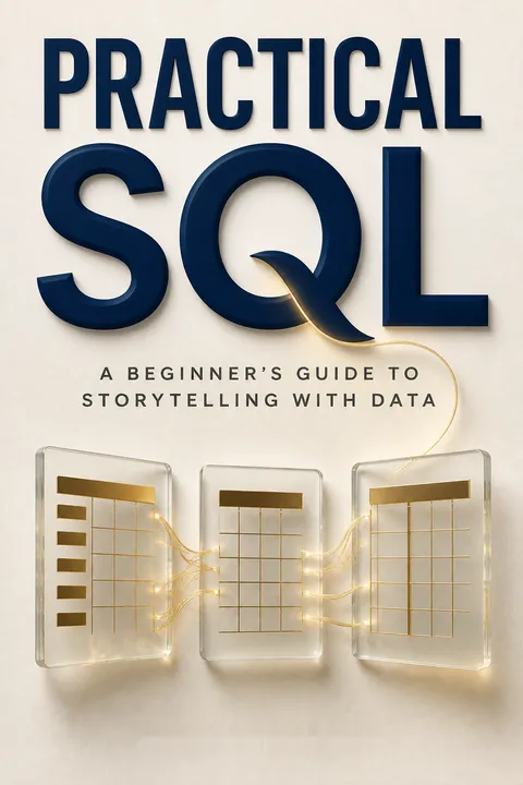
Practical SQL receives mostly positive reviews, with readers praising its clear explanations, practical examples, and comprehensive coverage of SQL concepts. Many find it helpful for beginners and as a refresher for experienced users. The book's focus on real-world datasets and data storytelling is appreciated. Some readers note the difficulty increases in later chapters, and a few struggle with PostgreSQL installation. Overall, it's considered a valuable resource for learning SQL and database management, with an average rating of 4.28 out of 5 based on 207 reviews.
People Also Read








Glossary
Interviewing the data
Initial data quality investigationA process of using queries to learn what a dataset contains, how its values are distributed, and whether records appear complete and consistent. Typical checks include counts, distinct values, minimums and maximums, filters for missing values, and joins that reveal unmatched keys. The goal is to understand a dataset's suitability before relying on it.
Natural key
Meaningful existing identifierA primary key built from one or more existing data fields whose values uniquely identify every row and are never missing. A product code or a combination of state and county codes may work as a natural key. Its advantage is that it carries real-world meaning; its risk is that the data may change or contain duplicates.
Surrogate key
Artificial row identifierA primary key added to a table when its real-world data does not provide a dependable unique identifier. It is commonly an automatically generated integer, though a UUID can also be used. A surrogate key remains independent of changes to descriptive data, but requires extra storage and does not itself explain what a row represents.
Common table expression (CTE)
Named temporary query resultA named result set defined with a WITH clause and available to the main query that follows. A CTE can make complicated SQL easier to read by separating preprocessing steps, such as grouping population by state before joining it to business counts. It exists for that query rather than as a permanent database table.
Window function
Calculation across related rowsA function that calculates a value for each row using a specified set of rows, without collapsing those rows into one aggregate result. The OVER clause defines the window, while ORDER BY or PARTITION BY can control its sequence or groups. Ranking and rolling averages are common examples.
Materialized view
Stored query resultsA database object that runs a query and stores its output as data, unlike a standard view, which runs its query when accessed. Stored results can make complex queries faster to read, but they do not automatically reflect changes in their source tables. A refresh reruns the query and updates the stored output.
tsvector
Normalized searchable textA PostgreSQL data type used to store text in a form suited to full-text search. Text is converted into normalized linguistic units called lexemes, often reducing inflected forms to a common root and omitting common stop words. The stored representation also records word positions, allowing search operators to match terms and their relationships.
Spatial reference system identifier (SRID)
Coordinate system identifierA numeric identifier for the coordinate reference system used by spatial data. Spatial operations often require objects to use compatible systems, and an SRID indicates how coordinates relate to locations on Earth or a projected map. In the examples, SRID 4326 identifies WGS 84, a widely used longitude and latitude system.
FAQ
What's Practical SQL: A Beginner's Guide to Storytelling with Data about?
- Focus on SQL Basics: Practical SQL introduces readers to SQL as a tool for data analysis, covering fundamental concepts and practical applications.
- Storytelling with Data: The book emphasizes using SQL to uncover insights and tell stories, making it relevant for journalists, analysts, and data enthusiasts.
- Hands-On Approach: Anthony DeBarros provides practical exercises and real-world examples, allowing readers to apply what they learn immediately.
Why should I read Practical SQL?
- Beginner-Friendly: Designed for those new to programming and SQL, it guides readers step-by-step through the learning process.
- Comprehensive Coverage: Covers a broad range of topics, including data types, importing/exporting data, and advanced querying techniques.
- Real-World Applications: Uses real datasets to illustrate concepts, making the learning experience relevant and engaging.
What are the key takeaways of Practical SQL?
- SQL Fundamentals: Learn the basics of SQL, including creating databases, tables, and performing queries.
- Data Manipulation Techniques: Master techniques like aggregation, filtering, and joining tables for effective data analysis.
- Best Practices: Emphasizes best practices in database design and data integrity, crucial for maintaining high-quality data.
What are the best quotes from Practical SQL and what do they mean?
- "SQL has been useful to me ever since.": Highlights the enduring value of SQL skills in various professional contexts.
- "Proper planning prevents poor performance.": Underscores the importance of setting up a solid foundation before diving into SQL coding.
- "Interviewing the data is exciting because you discover truths.": Reflects the author's perspective on data analysis as a process of exploration and discovery.
What is SQL and why is it important?
- Structured Query Language: SQL is used for managing and manipulating relational databases, allowing efficient data operations.
- Data Management: Crucial for data analysis, enabling users to extract insights from large datasets.
- Industry Standard: Widely used across industries, making it a valuable skill for job seekers in data-related fields.
How do I set up my coding environment for SQL?
- Install PostgreSQL: The book guides readers through installing PostgreSQL, a popular open-source database system.
- Use pgAdmin: Recommends using pgAdmin, a graphical interface for managing PostgreSQL databases, to simplify coding.
- Download Example Data: Encourages downloading example datasets from GitHub for hands-on practice.
What are the different types of JOINs in SQL?
- INNER JOIN: Returns only the rows where there is a match in both tables, useful for retrieving related data.
- LEFT JOIN: Returns all rows from the left table and matched rows from the right table, with NULLs for unmatched rows.
- FULL OUTER JOIN: Returns all rows from both tables, with NULLs where there is no match, useful for identifying discrepancies.
How do I import and export data using SQL?
- COPY Command: Explains using the COPY command to import data from a CSV file into a PostgreSQL table.
- Exporting Data: Learn to export data from a table to a CSV file using the COPY command.
- Handling Delimited Files: Discusses understanding delimited text files, including handling header rows and quoting columns.
What are aggregate functions in SQL?
- SUM and AVG: Perform calculations on a set of values in a column, essential for summarizing data.
- COUNT and MODE: COUNT counts the number of rows, and MODE identifies the most frequently occurring value.
- Using Percentile Functions: Introduces percentile functions like percentile_cont() for calculating medians and other quantiles.
How does Practical SQL approach data storytelling?
- Identifying Trends: Emphasizes identifying trends in data to tell a compelling story.
- Communicating Findings: Provides guidance on effectively communicating data findings to various audiences.
- Real-World Examples: Uses examples to illustrate how data storytelling can impact decision-making.
How does Practical SQL help with database management?
- Creating and Modifying Tables: Teaches how to create and modify database tables for effective management.
- Using Indexes: Covers the importance of indexes in improving query performance.
- Data Integrity: Discusses constraints and data validation techniques to ensure data integrity.
How can I apply the skills learned in Practical SQL to my job?
- Data-Driven Decision Making: Helps analyze data relevant to your job, leading to more informed decisions.
- Improving Efficiency: Mastering SQL can automate repetitive data tasks, saving time and reducing errors.
- Enhanced Communication: Focus on storytelling with data equips you to present findings clearly and persuasively.
Download PDF
Download EPUB
.epub digital book format is ideal for reading ebooks on phones, tablets, and e-readers.